Berkeley California Real Estate Market Research.
I analyzed Berkeley Real Estate Home Sales from the East Bay Regional (EBRDI) MLS/Berkeley Board of Realtors MLS Sales from 2007.
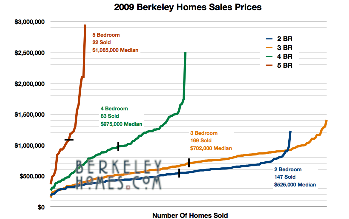
Click on the graph to go to the video I created to explain it all.

This video shows how the median (mid point – half the homes sold for more, half the homes sold for less) home sales price in Berkeley has changed from 2007 to Mid April 2010.
I’ve organized the data by bedrooms, price, median price … and also included a graph to show the effect that “days on the market” has on the sales price/original price ratio.
Most of the homes in Berkeley were built up in 1910 to 1920’s and have 2 & 3 bedrooms. One graph shows the relationship between the home’s square footage and sales price.
Note: EBRDI/Berkeley MLS does not reflect every home sale in Berkeley.

Interesting but hard to understand. Cumulative frequency graphs typically display the number of items on the Y axis.
See wikipedia http://en.wikipedia.org/wiki/Cumulative_frequency_analysis:
The cumulative frequency is the frequency with which the value of a variable Y is less than a reference value X. The cumulative frequency Fc(Y<X) is found from Fc(Y<X) = MX/N, where MX is the number of data Y with a value less than the reference value X, and N is the total number of data. Considering X as a variable, Fc(Y<X) can be called the cumulative frequency function or cumulative frequency distribution of Y. The previous expression may be briefly written as Fc = M/N.
As the minimum value of M is zero and the maximum is N, the value of Fc ranges between 0 and 1 or 100%
I’m always looking for ways to present information more clearly. I’ll be uploading a chart I created showing the distribution of homes sold in Berkeley as a function of price, which is one more way of viewing the data.